Moon Formation Simulation in Kotlin

This article presents a Kotlin n-body code that can model collisions between planets.

The algorithm may look daunting at first, but without the tree-code (which is optional), it's fairly simple, at around 400 lines of code.

In my opinion, n-body codes are a good mid-level project. There's a huge gap between what you get if you search for simple programming projects, and what you get if you do a PhD in computational physics, and projects like the one presented here are a good mid-level project, where code layout and structure become important (not that I've got that right), but you don't need to invest years of your life into getting results.

The code can be found here: https://github.com/hm123/abap_knbody

What happened

It is thought likely that the Moon was formed when a planet (we now call Theia) collided with the young Earth, about 4.4 billion years ago.

Scientists think this because:

• The moon has very similar isotope ratios to the earth:
• The moon is spiraling outward because it orbits more slowly than the Earth's spin, and is big enough to exert a tide on the Earth's oceans. If you rewind the clock, you eventually get back to a time when the moon was much closer to the Earth.
• Such a heavy object as the Moon would be extremely difficult to capture by the Earth in a nearby low orbit without a collision.
• Lots of other reasons. See here: https://en.wikipedia.org/wiki/Giant-impact_hypothesis

The sequence of events is probably:

• Theia collides with the Earth.
• A lot of junk gets thrown into orbit.
• Earth is spinning really fast as a result of the collision.
• Earth now has an extremely thick atmosphere of vaporised rock.
• The thick vaporised rock forms a thick disk or synestia (like a cross between a very thick disk, and a donut shaped thick atmosphere) around the Earth.
• Over a time on the timescale of years to centuries, a moon forms in orbit from this junk.

One fun project is to simulate the initial collision. To do this accurately is extremely difficult because you have to model solid / gas behaviour, temperature flows, gas / rock mixing, chemistry, small scale turbulence, etc., etc.

Fortunately, people have already done this, and so you can get some realism by doing the simulation extremely approximately, and then tweaking the parameters until it vaguely matches the accurate simulations. Obviously this isn't primary research any more, but it still allows you to obtain a working simulation of the collision with somewhere around a 7 days work, rather than 7 years.

The approach

(The code for these simulations is on GitHub: https://github.com/hm123/abap_knbody. I'll talk through the code briefly, but the interested reader should probably just read the code, since there are details I've omitted for brevity.)

The Earth is 1 planet. Theia is 1 planet. Between them they have somewhere around 7e24 kg of rock. We pretend that instead, they are composed of several thousand particles.

Each particle (p) is composed of three things: a position vector (p.p), a velocity vector (p.v) and a temperature (p.t) (purely for display at the moment). We say that these particles have to obey laws.

Physical laws are normally expressed using differential equations. Here they are instead using kotlin code, which does essentially the same thing.
Differential equations say that if the universe looks like X, the way the universe is changing is dX/dt = f(X).
A timestep function says that if the universe looks like X, then after time dt, the universe looks like X_after = f(X_before, dt).
These aren't identical ideas, but they're pretty similar.

Firstly, though, here's our simulation state:

class V3(var x:Double, var y:Double, var z:Double)
class P(val p : V3,val v: V3,var t:Double)
class State(val p:Array< P >, val m1:Double, val radius:Double)

The variable m1 is the mass of each particle in kg. The radius is the radius of each particle, in metres.
A object of type Sim, therefore, represents the state of the simulation. Our timestep function takes a sim, and changes it, in place, as if it was now time dt later.

We first initialise it with random positions for each particle.

The first law that the particles have to obey is that they move in the direction of their velocity. This can be expressed using the following timestep code:

class State(val p:Array< P >, val m1:Double, val radius:Double)
{
    fun timestep(dt:Double){
        timestepP(dt)
        timestepV(dt)
    }

    fun timestepP(dt:Double){
        for(particle in p) {
            particle.p.x += i.v.x * dt
            particle.p.y += i.v.y * dt
            particle.p.z += i.v.z * dt
        }
    }

    fun timestepV(dt:Double){
        for(i in 0 until p.size){
            for(j in 0 until i){
                pairInteraction(p[i],p[j],dt,radius,m1)
            }
        }
    }

// This function is used both by the N^2 and NLogN algorithms to model how two nearby particles interact.
// p1 is the first particle.
// p2 is the second particle.
// dt is the timestep length.
// radius is the radius of a particle in metres.
// m1 is the mass of 1 particle in kg.
// Note that this function writes out the vector calculations for speed
// It would be clearer if it used vector methods, but possibly take longer to run.

fun pairInteraction(p1: P, p2: P, dt: Double, radius:Double, m1:Double) {
    val p1p = p1.p
    val p2p = p2.p

    val p1v = p1.v
    val p2v = p2.v

    // This vector is the relative position of p2 to p1.
    val dx = p2p.x-p1p.x
    val dy = p2p.y-p1p.y
    val dz = p2p.z-p1p.z

    // This is the distance between the particles.
    val d = Math.sqrt(dx*dx+dy*dy+dz*dz + 0.0001 * radius*radius)

    // gravitational force (or will be when multiplied by (dx,dy,dz))
    val f = dt * (
            GRAV_CONST * m1 / (d*d*d)
            )

    // now convert to a force.
    val fx = dx * f
    val fy = dy * f
    val fz = dz * f

    // now update the velocities.
    p1v.x+=fx
    p1v.y+=fy
    p1v.z+=fz
    p2v.x-=fx
    p2v.y-=fy
    p2v.z-=fz

    if (d < radius){

        // normalised direction between particles.
        val wx=dx/d
        val wy=dy/d
        val wz=dz/d

        // relative velocity of v2 to v1.
        val dvx = p2v.x - p1v.x
        val dvy = p2v.y - p1v.y
        val dvz = p2v.z - p1v.z

        // collision speed.
        val vd = (wx*dvx+wy*dvy+wz*dvz)

        // update temperature of particles.

        p1.t+=vd*vd*0.010
        p2.t+=vd*vd*0.010

        p1.t*=0.9
        p2.t*=0.9

        if (vd < 0) {
            piv.x +=wx * vd
            piv.y +=wy * vd
            piv.z +=wz * vd
            pjv.x -=wx * vd
            pjv.y -=wy * vd
            pjv.z -=wz * vd
        }

    }
}

To summarise the step above, you:

• Update the positions using the current velocity.
• For every pair of particles:
  • Add a gravitational attraction between them
  • If they're closer together than radius, add an outward force pushing them apart.
  • If they're closer together than radius and are moving toward each other, then bounce them: However fast they were moving towards each other, they are now moving apart.

The timestep there is really simple, and it's clearly not going to be all that accurate since country-sized spheres of rock don't bounce like this in real life, but it's close enough that the basic shape of a planetary collision sort-of works.

Another point is that it seems odd to update the positions first, then velocity second, when we could update both at the same time. It turns out that doing the two update steps separately is more accurate over the long term, because the steps are reversible (except for the bounce part). If you reverse the velocities, and then run the same timestep process (and ignore a tiny detail), the simulation would run backwards.

Because the simulation runs forward and backward with the same simulation code, it means that it is unlikely to be introducing a long-term drift to the energy.

(To rephrase, imagine that there was a positive long-term drift. Now reverse the velocities. Do we have a positive long-term drift because our timestep is positive-drift, or do we have a negative because we're running it backward? The only way to resolve this paradox is to conclude that there's no simple long term drift term).

How well does this work? Here's a simulation with 3000 particles:

(By the way, all simulations are at 300x speed, so 12 seconds = 1 hour)

Performance

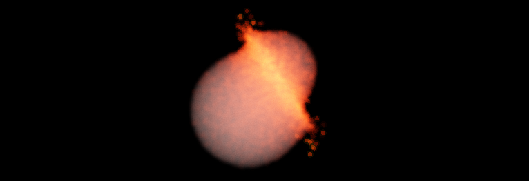
The code above works, but the time it takes to update the simulation is proportional to the number of particles squared. This means that it works perfectly well for 3000 particles, taking perhaps 10 minutes.

If you want to run for 50000 particles, it takes 300 times as long: 3000 minutes or several days.

You can improve upon that using something that considers groups of particles far apart as the same particle. . This takes time (at least in theory) proportional to NlogN, and has about the same time (for me at least) at around 3000 particles.

(In the code, it's here: here)

That allows much larger simulations, like the following:

(Another sim with slightly different parameters is here.)

Accuracy

So ... we have a simulation of 50k particles crashing together in a way that, arguably, *looks* realistic.

How useful is that? If you're writing a blog post about the moon's formation in Kotlin, pretty useful.

But how accurate is this? The answer is that there's no reason to expect it to be all that accurate... but let's see:

• Gravity: This is almost exactly right, depending on the approximations in the tree code.
• Are we modelling a fluid: Yes: This many points all acting with local forces, seems to behave like a fluid.
• Does the fluid have the right properties: No...
  • Speed of sound: far too high
  • Compressibility: too low (related to above)
  • Does it vapourise: no. The real collision probably had clouds of rock vapour billowing everywhere. This one doesn't.
  • Viscosity: probably too high: Real life may have had a more "splashy" collision. In particular, you can see that the remaining earth is no longer round after the collision. That's because in this simulation, the stuff is too strong, and too viscous.
  • Do we handle heating properly: no. We don't.
  • Turbulence: In this sim, there's not much turbulence. In real life, there might well be lots.

Also, I haven't really put that much effort into getting the initial conditions (masses of planets, angle of attack, speed) right.

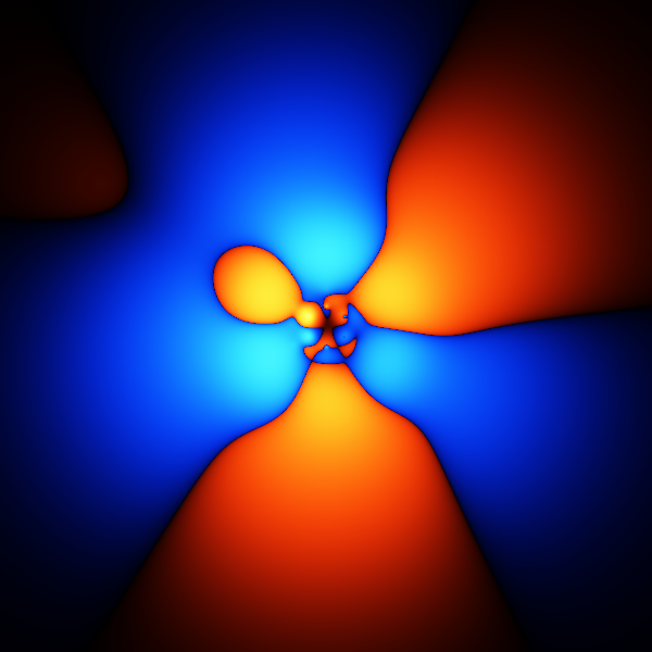
More compressible version

To see how much difference all the things above make, let's try a completely different model of how particles might interact:

// This function is used both by the N^2 and NLogN algorithms to model how two nearby particles interact.
// p1 is the first particle.
// p2 is the second particle.
// dt is the timestep length.
// radius is the radius of a particle in metres.
// m1 is the mass of 1 particle in kg.
// Note that this function writes out the vector calculations for speed
// It would be clearer if it used vector methods, but possibly take longer to run.

fun pairInteraction(p1: P, p2: P, dt: Double, radius:Double, m1:Double) {
    val p1p = p1.p
    val p2p = p2.p

    val p1v = p1.v
    val p2v = p2.v


    // This vector is the relative position of p2 to p1.
    val dx = p2p.x-p1p.x
    val dy = p2p.y-p1p.y
    val dz = p2p.z-p1p.z

    // This is the distance between the particles.
    val d = Math.sqrt(dx*dx+dy*dy+dz*dz + 0.0001 * radius*radius)

    // gravitational force (or will be when multiplied by (dx,dy,dz))
    val f2 = dt * (
            GRAV_CONST * m1 / (d*d*d)
            )
    // add in an outward force for particles too close.
    val g = f2 + dt * Math.min(0.0,d - 2.00*radius)/(radius*d) * RESTORING_FORCE

    // now convert to a force.
    val fx = dx * g
    val fy = dy * g
    val fz = dz * g

    // now update the velocities.
    p1v.x+=fx
    p1v.y+=fy
    p1v.z+=fz
    p2v.x-=fx
    p2v.y-=fy
    p2v.z-=fz

    // This is just so that the energy of each collision affects the colour of
    // the particle:
    if (d < radius * 2.0){

        // normalised direction between particles.
        val wx=dx/d
        val wy=dy/d
        val wz=dz/d

        // relative velocity of v2 to v1.
        val dvx = p2v.x - p1v.x
        val dvy = p2v.y - p1v.y
        val dvz = p2v.z - p1v.z

        // collision speed.
        val vd = (wx*dvx+wy*dvy+wz*dvz)

        // update temperature of particles.

        p1.t+=vd*vd*0.010
        p2.t+=vd*vd*0.010

        p1.t*=0.9
        p2.t*=0.9

        // Old code that handled collisions.
        /*

        if (vd < 0) {
            piv.x +=wx * vd
            piv.y +=wy * vd
            piv.z +=wz * vd
            pjv.x -=wx * vd
            pjv.y -=wy * vd
            pjv.z -=wz * vd
        }

        */

    }
}

I've also slowed the collision down a bit, matching two planets on more-or-less the same orbit colliding.

You can see that it's a lot more "splashy", and this time a visible shock wave propagates through both planets.

Is this more accurate? Perhaps yes, perhaps no. Either way, it gives an indication of how accurate these models are, knowing that neither simulation is more likely than the other to be what actually happened.

This particular sim (above) lacks one key thing: Basically no stuff ends up in orbit, so no Moon.

Let's try running that again with more angular momentum and a slightly faster collision:

(Simulation finished)

Epilogue

The simulations above only really cover the first few hours after the simulation. After that, the orbiting stuff forms a thick ring around the rapidly rotating planet, possibly forming a synestia where the surface, the atmosphere and the ring all become mixed in a donut shape.

From this, a moon can form -- not too close, because tidal forces would rip it apart. It then gathers material to it, over the following years and centuries.

---

Other Articles:

---

© Hugo2015. Session @sessionNumber