Quantum mechanics for programmers
My main article on quantum mechanics is here. This article talks about how to make simulations like the ones there. For the actual simulations, I used C#, because it's a good compromise between speed and simplicity. I regret, sometimes, that it's not as fast as C, but it's easier to debug, and that saves me a lot of time. I'm going to try to explain how to do the simulations in Javascript, because it's easier to share with readers, and it means that you can play with the simulations in your browser. The disadvantage of javascript is that it's a bit slower. Normally it's only a factor of 2-10 times slower, but the slow bit in the simulations below is the fourier transform. For non-javascript languages, you use someone else's fourier transform library, and they're much faster because they use all the tricks that modern computers allow, from ordering operations optimally to making sure caches are used as well as possible. My javascript version? Not so much. The result is that the javascript version below is actually a *lot* slower than the C# version. Article aims:- To give a really simple simulation of a quantum mechanics system so that people who already know javascript have a chance to "get" quantum mechanics without necessarily having to understand the equations. The equations will help, though.
- To answer the question of "how do you make the simulations".
Quantum mechanics can be simulated with quite simple programs. Understanding what they do might help learn quantum mechanics, and it might help physicists understand how to simulate the maths. This article is going to start easy and get harder. If it's too easy, skip ahead.
Starting point: Euler
Here's the Schrödinger equation for a 1-D electron in a harmonic potential. Whether or not you understand it is ok, hopefully the article will be readable either way. $$i \frac{\partial \psi}{\partial t} = -\frac{\partial^2}{\partial x^2}\psi + ax^2\psi.$$ Let us rewrite that, introducing a timestep time, $\delta t$ $$\psi_{\hbox{after timestep}} \simeq \psi_{\hbox{before}} - i \delta t \left(-\frac{\partial^2 }{\partial x^2}\psi + ax^2\psi\right).$$ You can write $$\frac{\partial^2 }{\partial x^2}\psi(x) \simeq \frac{ \psi(x+1) - 2 \psi(x) + \psi(x-1) }{\delta x^2}.$$ These two approximations give us a simple timestepping function. This is not the only (or best) timestepping function that solves the problem, but perhaps it's one of the simplest. You, the reader, should try to understand the function below. Hopefully, it will make sense with the two equations above.
        // This returns an empty wavefunction of length n.
        function wavefunction(n){
            var psi = [];
            for(var i = 0; i < n; i++){
                psi[i] = {real: 0, imag: 0}
            }
            return psi; // for example [{real:0, imag:0}, {real:0, imag:0}, ...]
        }
        // This takes the starting wavefunction, and returns the wavefunction a short time later.
        function timestep(psi)
        {
            // This is how many units of time we're going to try to step forward.
            var dt = 0.002;
            var n = psi.length;
            // This is the wavefunction we're going to return eventually.
            var ret = wavefunction(n);
            // We miss off the first and last elements because it looks at the element to the
            // left and right of this point.
            for(var i = 1; i < n-1; i++)
            {
                // This is the x that is in the equation above.
                var x = (i-n/2)
                // This is the potential at this point.
                var V = x*x * 0.0015; // a here = 0.0015
                // We start from the original wavefunction (and later add (dt * dpsi/dt) to it).
                ret[i].real = psi[i].real;
                ret[i].imag = psi[i].imag;

                // This is the kinetic energy applied to psi.
                var KPsi = {
                    real: psi[i].real * 2 - psi[i-1].real - psi[i+1].real,
                    imag: psi[i].imag * 2 - psi[i-1].imag - psi[i+1].imag
                };
                // This is the potential, applied to psi
                var VPsi = {
                    real: psi[i].real * V,
                    imag: psi[i].imag * V
                };
                // This is the whole right hand side of the schrodinger equation.
                var rhsReal = KPsi.real + VPsi.real;
                var rhsImag = KPsi.imag + VPsi.imag;
                // This adds it, multiplied by dt, and multiplied by i.
                // The multiplication by i is what swaps the real and imaginary parts.
                ret[i].real += rhsImag * dt;
                ret[i].imag -= rhsReal * dt;
            }
            return ret;
        }

        // This returns the initial state of the simulation.
        function init(){
            var n = 128;
            var psi = wavefunction(n);
            for(var i = 0; i < n; i++){
                psi[i].real = Math.exp(-(i-20)*(i-20)/(5*5))*0.75;
                psi[i].imag = 0;
            }
            return psi;
        }
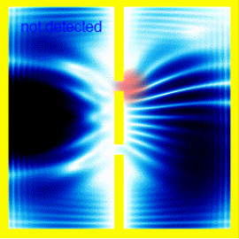
The simulation above is the probability density of an electron in an $x^2$ potential.
This is similar to if it was in a bowl, and was rolling backwards and forwards in that bowl.
The simulation works, but it has problems:
- The total amount of probability grows with time.
- If you time the oscillation, it's not quite right: It's actually moving slightly too slowly when it's at its fastest
- There's dispersion: The oscillation doesn't stay focussed. It should: this particular potential is specially chosen to make the oscillation stay focussed.
Split operator
This is going to get harder quickly. Let's start withWe're going to have to look at the original equation again.
A different way to convert it into a timestep is to do this.
$$\psi_2 = \hbox{Timestep}_T(\psi_1)$$ $$\psi_1 = \hbox{Timestep}_V(\psi_0)$$
Here, $\psi_0$ is the wavefunction before the timestep.
$\hbox{Timestep}_V$ steps forward with according to the following equation: $$i \frac{\partial \psi}{\partial t} = ax^2\psi.$$
$\hbox{Timestep}_T$ steps forward with according to the following equation: $$i \frac{\partial \psi}{\partial t} = -\frac{\partial^2}{\partial x^2}\psi$$
$\hbox{Timestep}_V$ is actualy really easy to implement, because: $$\hbox{Timestep}_V(\psi) = e^{-iax^2\delta t}\psi.$$
$\hbox{Timestep}_T$ can be implemented by noting that if $\psi = e^{ikx}$, then: $$\hbox{Timestep}_T(\psi) = e^{-ik^2\delta t}\psi.$$
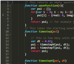
And there's good news: We can implement this by fourier transforming, then multiplying by $e^{i k^2}$, and then inverse fourier transforming. The fourier transform code is here:FFT.js. This particular fourier transform code only works on powers of two.
        // This returns an empty wavefunction of length n.
        function wavefunction(n){
            var psi = [];
            for(var i = 0; i < n; i++){
                psi[i] = {real: 0, imag: 0}
            }
            return psi; // for example [{real:0, imag:0}, {real:0, imag:0}, ...]
        }
        // This takes the starting wavefunction, and returns the wavefunction a short time later.
        function timestep(psi)
        {
            // This is how many units of time we're going to try to step forward.
            var dt = 0.02;
            psi = timestepV(psi, dt);
            psi = timestepT(psi, dt);
            return psi;
        }

        function timestepV(psi, dt)
        {

            var n = psi.length;
            for(var i = 0; i < n; i++)
            {
                // This is the x that is in the equation above.
                var x = (i-n/2)
                // This is the potential at this point.
                var V = x*x * 0.0015;
                var theta = dt * V;
                var c = Math.cos(theta);
                var s = Math.sin(theta);
                var re = psi[i].real * c - psi[i].imag * s;
                var im = psi[i].imag * c + psi[i].real * s;
                psi[i].real = re;
                psi[i].imag = im;
            }
            return psi;
        }

        function timestepT(psi, dt){
            psi = FFT.fft(psi);
            var n = psi.length;
            for(var i = 1; i < n/2; i++)
            {
                var k = 2 * 3.1415927 * i / n;
                var theta = k * k * dt;
                var c = Math.cos(-theta);
                var s = Math.sin(-theta);
                var re = psi[i].real * c - psi[i].imag * s;
                var im = psi[i].imag * c + psi[i].real * s;
                psi[i].real = re;
                psi[i].imag = im;


                var j = n - i;
                re = psi[j].real * c - psi[j].imag * s;
                im = psi[j].imag * c + psi[j].real * s;
                psi[j].real = re;
                psi[j].imag = im;

            }
            return FFT.fft(psi);
        }
        // This returns the initial state of the simulation.
        function init(){
            var n = 128;
            var psi = wavefunction(n);
            for(var i = 0; i < n; i++){
                psi[i].real = Math.exp(-(i-20)*(i-20)/(5*5))*0.75;
                psi[i].imag = 0;
            }
            return psi;
        }
This runs much better. It's faster, mainly because the timestep was longer. But the timestep can be longer
because the timestep is more accurate. Likewise, you can get away with a coarser grid, and still get the same accuracy.
The next page looks at 2-dimensional simulations:
Here
Other Articles:
|
The double slit and observersA look at the double slit experiment. The first half is meant to be a clear explanation, using simulations. The second half discusses some of the philosophy / interpretations of quantum mecahnics. |
|
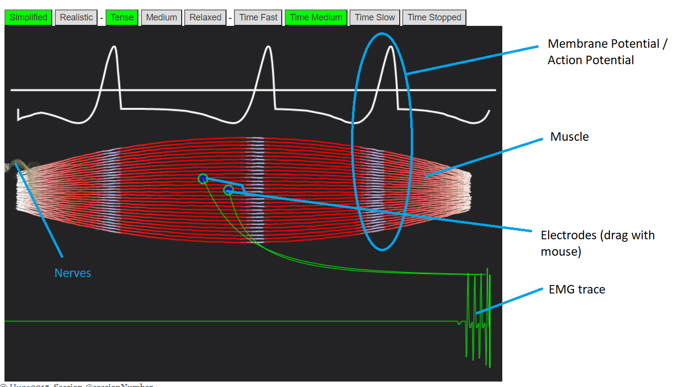
BodyWorks: Neuromuscular Activity / Muscle EMGAn interactive simulation showing how nerves travel to and down muscles, and how this gets picked up by EMG sensors. |
|
Quantum Mechanics for programmersA quick demo showing how to make simulations of simple quantum mechanics systems in javascript. |